Deriving the Noise Gain vs Signal Gain of the Inverting Op Amp

Meanwhile, at the electronics lab, someone kept trying to analyze Walter Jung’s op-amp circuits using dream interpretation… 😆

How do we quantify the error effects of finite gain? Even in an otherwise ideal op-amp, the finite open-loop gain introduces deviations from the ideal as seen in the closed-loop gain equation. Using Jung’s IC Op Amp Cookbook and Roberge’s Operational Amplifiers: Theory and Practice, we can gain valuable insights from the derivation of the closed loop gain result for the inverting amplifier:

$$A_v=-\frac{R_f}{R_{in}}\frac{1}{1+1/(A_{vo}\beta )}$$

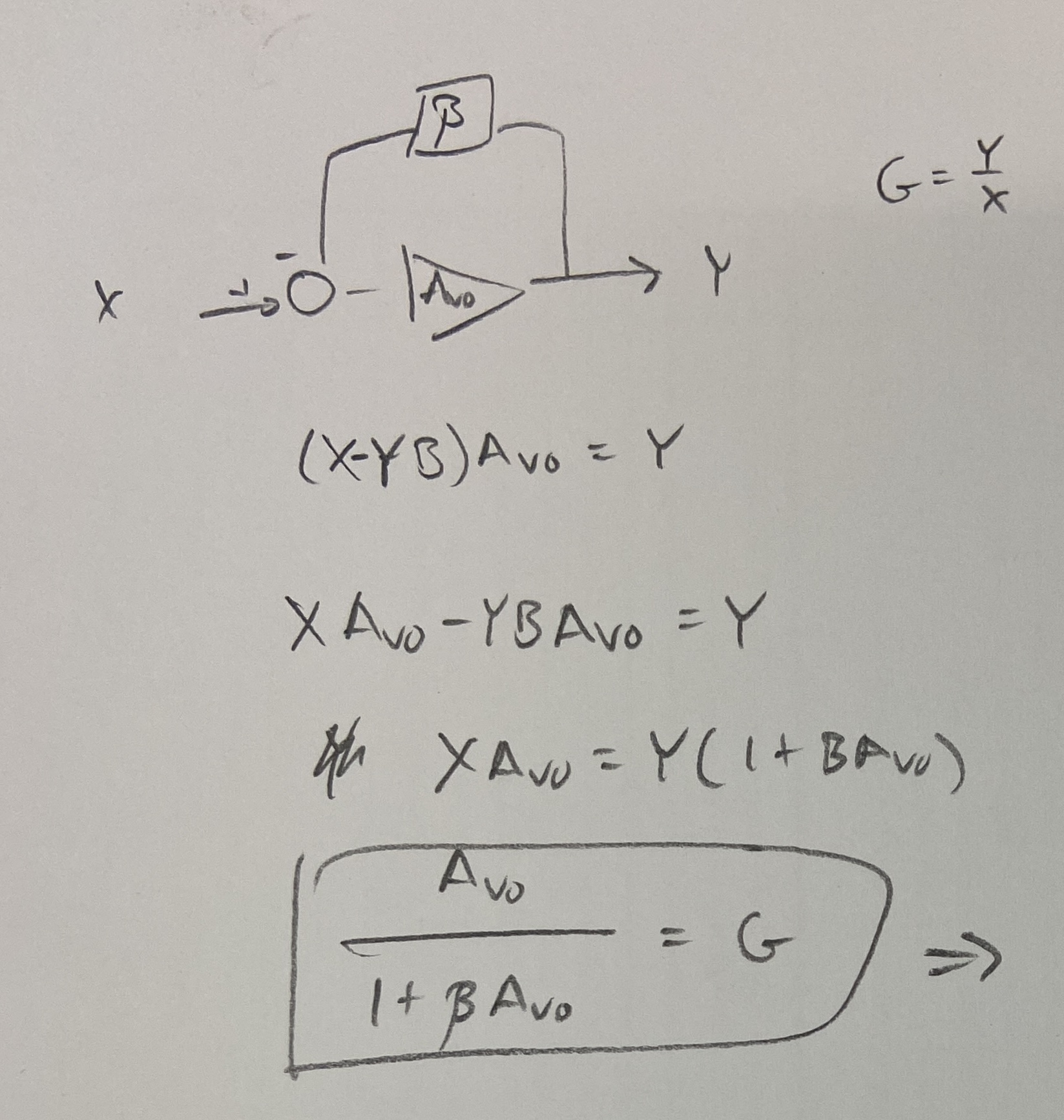
First, we define a term, $\beta$ , as the amount of output that is fed back to the input. Interestingly, we then identify $\frac{1}{\beta }$ as the “noise gain”, which is common for both non-inverting and inverting configurations. We will see, through the manipulation of the closed loop gain equation, why we call this the “noise gain”.

We can then analyze the closed loop gain in terms of the open loop gain and this $\beta$ term, noting how for high open loop gain $A_{vo}$ we get a closed loop gain equal to $\frac{1}{\beta }$ which is determined by components external to the op-amp. This is the key to ideal op-amp behavior - a very high open loop gain means we can just set the system gain using external components.

In Jung’s industry classic [1], Section 1.2.1 “Errors Due to Finite Open-Loop Gain”, he presents an equation for the closed loop gain of the inverting amplifier:

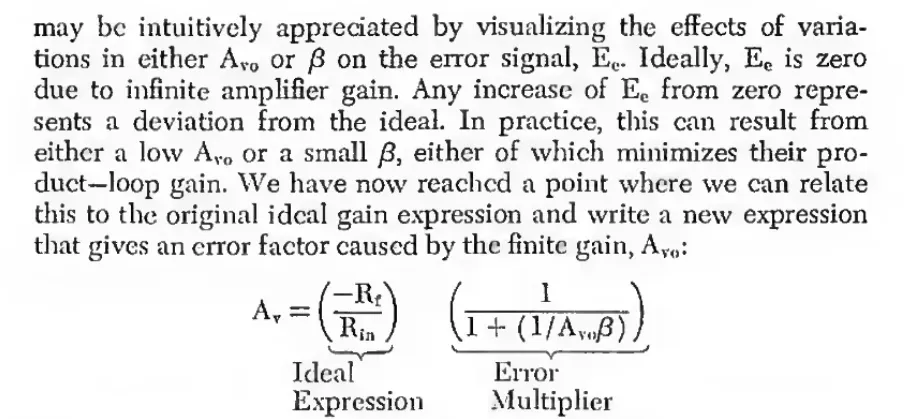
But it is not clear how he separates the ideal expression from the error multiplier terms. Clarity can be found by referencing the Roberge text [2] (available freely online).

For the inverting amplifier configuration, assuming no current flows into the op-amp, we can solve for the closed loop gain via superposition (see text):

$$A_v=-\frac{A_{vo}{Z}_2/(Z_1+Z_2)}{1+[A_{vo}{Z}_1/(Z_1+Z_2)]}$$

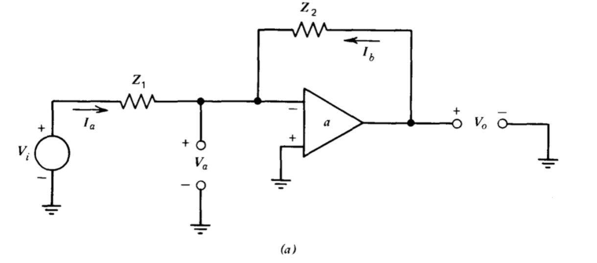
Then with some algebraic manipulations, we can finally derive the Jung equation. Since $\beta =\frac{Z_1}{Z_1+Z_2}$:

$$\begin{array}{rl}{A}_v& =-\frac{A_{vo}{Z}_2/(Z_1+Z_2)}{1+[A_{vo}{Z}_1/(Z_1+Z_2)]}\\ & =-\frac{A_{vo}{Z}_2/(Z_1+Z_2)}{1+A_{vo}\beta }\\ & =-\frac{Z_2}{Z_1+Z_2}\frac{A_{vo}}{1+A_{vo}\beta }\\ & =-Z_2\frac{\beta }{Z_1}\frac{A_{vo}}{1+A_{vo}\beta }\\ & =-\frac{Z_2}{Z_1}\frac{1}{1+1/(A_{vo}\beta )}\end{array}$$

Where the $\frac{-Z_2}{Z_1}$ term is the one we expect for the ideal inverting amplifier. Thus the other term is an error term depending on $A_{vo}\beta$. For small values of $A_{vo}\beta$, this error term becomes less than 1, decreasing our overall gain.

This shows the effects of non infinite open loop gain of the op-amp. This actually becomes important at higher frequencies as the open loop gain of the op-amp itself decreases and the $A_{vo}\times \beta$ starts to play more of a role.

For example, the LM738 op-amp gives an open loop gain of 100dB = 100,000 at DC which is down to 60dB = 1,000 at 1kHz. if $Z_2=100k$ and $Z_1=1k$ (ideal G = 100) then our error due to finite gain is around -9%. If we try to increase $G_{ideal}=\frac{Z_2}{Z_1}$ further to 1,000, we see our error increases to -50%! Since the open loop gain decreases at higher frequencies, the error in the closed loop gain increases.

References

[1] W. G. Jung, IC Op-Amp Cookbook, 1st ed., 2nd printing. Indianapolis, IN: Howard W. Sams, 1976.

[2] B. Roberge, Operational Amplifiers: Theory and Practice. New York: Wiley, 1976. Available freely online.

P.S. Bonus: You can put this knowledge to use for single ended to differential output conversion with fully differential amplifiers.